Expectation-Maximization
In this post, I reproduce many of the ideas (and some content) from the excellent textbook ‘Pattern Recognition and Machine Learning’ by Christopher M. Bishop.
Maximum Likelihood Estimation (MLE)
Given some some samples \(X\) from a distribution, we want to find out parameters \(\theta\) describing this distribution that maximize the likelihood of generating these samples, ie, \(p(X \mid \theta)\). For very simple distributions (such as a single Gaussian), this can often be solved in closed-form: differentiation of the likelihood with respect to \(\theta\) is enough.
However, this will not work for more complicated distributions (such as mixtures of Gaussians). Instead of closed-form solutions, we turn to iterative algorithms that can converge to atleast local maxima of the likelihood.
An example of an iterative approach which provably increases (rather, does not decrease) the likelihood at each step is Expectation-Maximization.
Expectation-Maximization (EM)
EM splits the log-likelihood (equivalent to the likelihood for maximization) into two terms, explicitly listing latent variables \(Z\). Latent variables are not observed, but if we had values for them, maximization of the log-likelihood is much simpler. In the case of mixture models, the latent variables for each sample \(x \in X\) would be the one-hot vector indicating which distribution in the mixture this sample was generated from.
The problem is that we don’t know the distribution of latent variables. The way EM tackles this is to compute a distribution of latent variables from our current estimate of the parameters! In simplified terms, EM consists of two steps, repeated until convergence:
- Compute distribution \(q\) over latent variables, with our current estimate of parameters \(\theta\).
- Compute new estimates of \(\theta\), using \(q\).
Start by specifying the joint distribution over both data \(X\) and latent variables \(Z\): \[ \begin{aligned} p(X, Z \mid \theta) &= p(X \mid \theta)\cdot p(Z \mid X, \theta) \newline \ln{p(X, Z \mid \theta)} &= \ln{p(X \mid \theta)} + \ln{p(Z \mid X, \theta)} \newline \end{aligned} \] Integrate with respect to some distribution \(q\) over latent variables \(Z\): \[ \int q(Z) \ln{p(X, Z \mid \theta)} \ dZ = \int q(Z) \ln{p(X \mid \theta)} \ dZ+ \int q(Z) \ln{p(Z \mid X, \theta)} \ dZ \] As \(\ln{p(X \mid \theta)}\) is independent of \(Z\), and \(q\) is a distribution: \[ \begin{aligned} \int q(Z) \ln{p(X, Z \mid \theta)} \ dZ &= \ln{p(X \mid \theta)} + \int q(Z) \ln{p(Z \mid X, \theta)} \ dZ \newline \int q(Z) \ln{p(X, Z \mid \theta)} \ dZ - \int q(Z) \ln{q(Z)} \ dZ &= \ln{p(X \mid \theta)} + \int q(Z) \ln{p(Z \mid X, \theta)} \ dZ - \int q(Z) \ln{q(Z)} \ dZ \newline \int q(Z) \ln{\left(\frac{p(X, Z \mid \theta)}{q(Z)}\right)} \ dZ &= \ln{p(X \mid \theta)} + \int q(Z) \ln{\left(\frac{p(Z \mid X, \theta)}{q(Z)}\right)} \ dZ \newline \end{aligned} \]
We assume continuous latent variables here, but the same steps hold for discrete latent variables (this is what is done in the reference); just replace integrals by sums.
If we define (the conditional density of \(Z\) given \(X, \theta\)): \[ p_{z, \theta}(Z) = p(Z \mid X, \theta). \] we see that the second term on the RHS is just the negative of the KL-divergence \(KL\left(q \ \middle\| \ p_{z, \theta} \right)\). (Note that \(X\) is going to be constant, as it represents our data which is completely known to us. Missing values would be considered as a latent variable, so those would be considered in \(Z\).) If we now define the evidence lower bound \(L\): \[ L(q, \theta) = \int q(Z) \ln{\left(\frac{p(X, Z)}{q(Z)}\right)} dZ \] then, we can summarize the equation as: \[ \ln p(X \mid \theta) = L(q, \theta) + KL\left(q \ |\middle| \ p_{z, \theta} \right) \]
To maximize the log-likelihood \(\ln p(X \mid \theta)\), EM does the following:
- E-step: Fix \(\theta\). Update \(q\) such that \(L(q, \theta)\) is maximized.
- M-step: Fix \(q\). Update \(\theta\) such that \(L(q, \theta)\) is maximized.
Both steps are guaranteed to increase (or atleast, not decrease) the evidence lower bound. As the KL-divergence is always non-negative, the log-likelihood will also not decrease.
The E-step
We have fixed \(\theta\) as \(\theta^{\ old}\). Note that \(\ln p(X \mid \theta^{\ old})\) is independent of latent variables \(Z\) (they have been marginalized out), so maximizing \(L(q, \theta^{\ old})\) is equivalent to minimizing \(KL\left(q \ \middle\| \ p_{z, \theta^{\ old}} \right)\). This occurs when \(q\) is exactly \(p_{z, \theta^{\ old}}\), and the \(KL\)-divergence becomes \(0\).
Thus, the E-step is basically computing \(p_{z, \theta^{\ old}}\). Why is this called the E-step? Let us define: \[ Q(\theta, \theta^{\ old}) = \mathop{\mathbb{E}}\limits_{Z \sim p_{z, \theta^{\ old}}}[\ln{p(X, Z \mid \theta)}] \]
It is clear that once we have computed \(p_{z, \theta^{\ old}}\), we can compute \(Q(\theta, \theta^{\ old})\) for any \(\theta\) supplied to us, by computing the expectation of some complicated term.
The M-step
We have fixed \(q\) as \(p_{z, \theta^{\ old}}\). Again, we want to maximize the evidence lower bound \(L\). Let us exactly list out what \(L\) is for an arbitrary \(\theta\), once we’ve fixed \(q\): \[ L(q, \theta) = \int q(Z) \ln{\left(\frac{p(X, Z \mid \theta)}{q(Z)}\right)} \ dZ = \int q(Z) \ln{p(X, Z \mid \theta)} \ dZ - \int q(Z) \ln{q(Z)} \ dZ \] But wait! Once we’ve fixed \(q\), the second term is a constant. The term that remains is: \[ \int q(Z) \ln{p(X, Z \mid \theta)} \ dZ = \int p_{z, \theta^{\ old}} \ln{p(X, Z \mid \theta)} \ dZ = \mathop{\mathbb{E}}\limits_{Z \sim p_{z, \theta^\ {old}}}[\ln{p(X, Z \mid \theta)}] = Q(\theta, \theta^{\ old}) \]
Thus, maximizing \(L\) subject to \(q\) fixed to \(p_{z, \theta^{\ old}}\), is the same as maximizing \(Q\) (as a function of \(\theta\)).
So, in the E-step, we compute \(Q\) which an expected value of some quantity, and in the M-step, we maximize \(Q\).
EM for MAP Estimation
EM can also be used for MAP (maximum a posteriori) estimation, the procedure is almost the same! In comparison with ML (maximum likelihood) estimation, MAP estimation chooses \(\theta\) maximizing the posterior distribution of parameters conditional on the input: \[ p(\theta \mid X) = \frac{p(X \mid \theta) \ p(\theta)}{\sum_\theta p(X \mid \theta) \ p(\theta)} \] Note, that the denominator is independent of \(\theta\). Hence, this is equivalent to maximization of: \[ p(X \mid \theta) \ p(\theta), \] which is the likelihood function multiplied by the prior distribution over parameters. Applying logs, we see that we have an additional additive term coming from the prior distribution: \[ \ln{p(X \mid \theta)} + \ln{p(\theta)} \]
Thus, the E-step (when \(\theta\) is fixed) is the same, because we have just added a constant (with respect to \(q\))! The M-step is slightly different, we now have to maximize: \[ Q(\theta, \theta^{\ old}) + \ln{p(\theta)} \]
EM is not (completely) Bayesian!
Why? A fully Bayesian technique would introduce distributions over the unknown parameters \(\theta\). EM does compute a distribution over latent variables \(Z\), but a gives us point estimate for \(\theta\) (and not a full distribution, irrespective of whether we use ML or MAP estimation). This last point might be a little confusing: I have written down the expressions for the posterior distribution of \(\theta\) in the section above! But, that distribution is often intractable. (Indeed, if it were tractable, so would the likelihood itself, which means we wouldn’t have to do EM anyways.)
However, once we specify a prior distribution over \(\theta\), we can now integrate \(\theta\) into the set of latent variables \(Z\). This merges the E- and M-steps! We will expand on this when we look at variational inference, in a future post.
An Example
The reference above discusses an example of EM for Gaussian Mixture Models really well. Take a look if you’re interested. Here, I will use their results and implement the E- and M-steps.
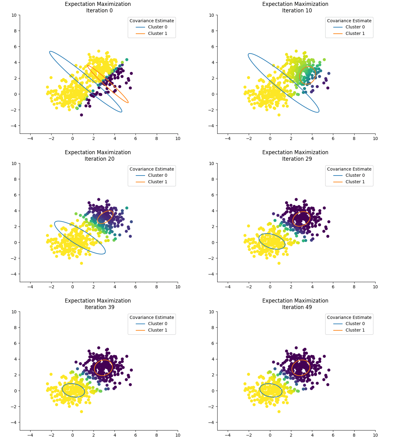
It is important to note that EM is susceptible to local maxima of the log-likelihood. Initializing by running k-means (which is actually a special case of EM!) first is a good idea. In the example below, I do not initialize the mixing coefficients and the means randomly, because I want to show how the estimates change:

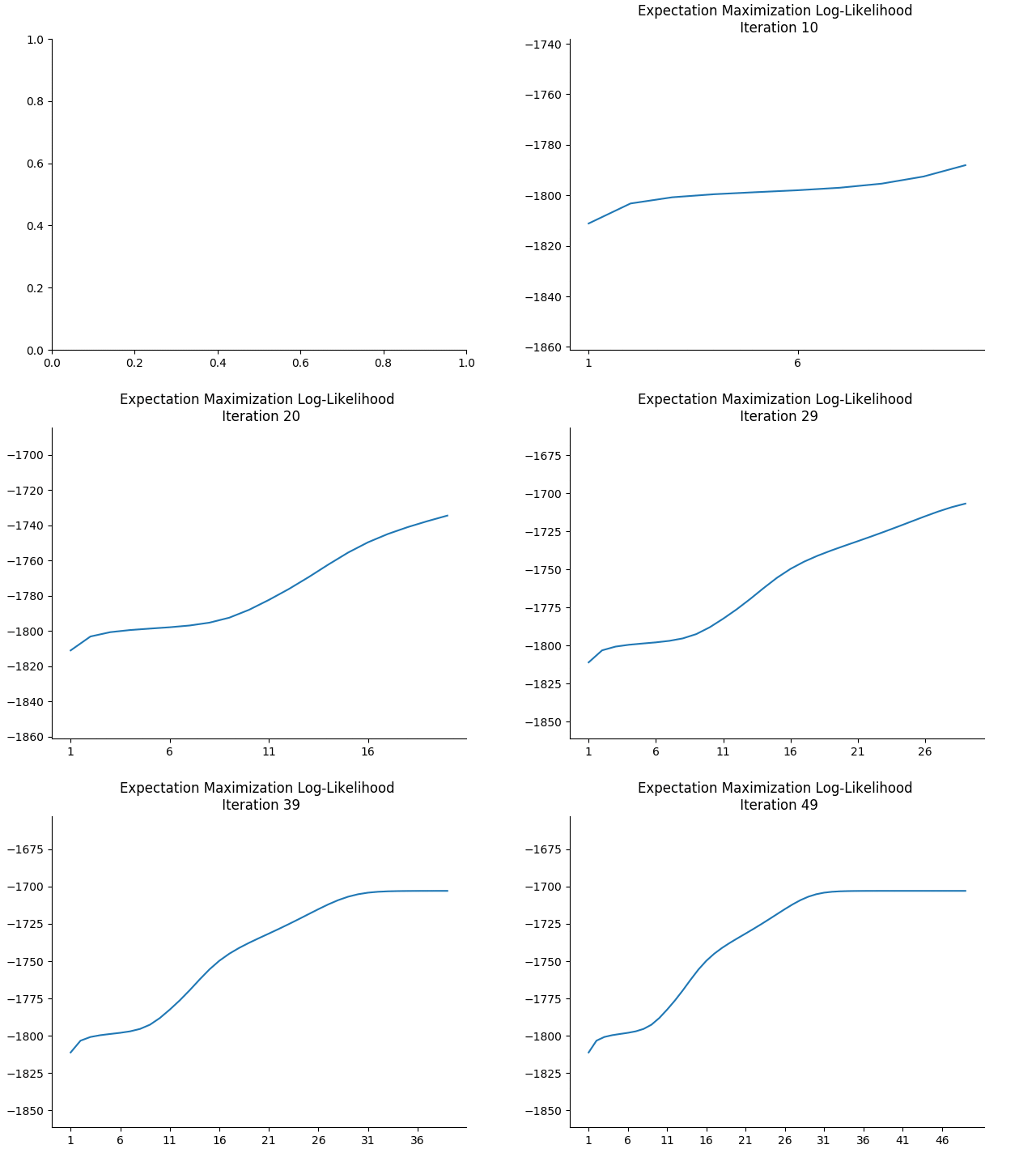
The colours for each sample indicate the responsibility of cluster 0 in ‘explaining’ that sample. If we plot the log-likelihoods after each iteration, we see that it is, indeed, non-decreasing:

I skip the initial log-likelihood in the plot above because it skews the plot, being very low.
In general, there is much to be said about the difficulty of implementing the E and M steps: for some models (such as Gaussian Mixture Models) both are relatively simple, but they can be complex (and even intractable). The reference has a great discussion about this, too.
The next post is to take this background and step into variational inference!
I’m also starting to introduce a commenting facility via GitHub Issues, in order to not clutter up this space here. Comment here!